massProps

Overview

The massProps package extends rollupTree with functions to recursively calculate mass properties (and optionally, their uncertainties) for arbitrary decomposition trees. Formulas implemented are described in a technical paper published by the Society of Allied Weight Engineers (Zimmerman and Nakai 2005).

Synopsis

Data Structures

massProps operates on two fundamental data structures: a mass properties table and a tree. The mass properties table has an entry for every item in a tree structure of items; the edges of the tree convey the parent-child relations among items. The two data structures are linked by the id column of the data frame, which must be a character vector of unique item identifiers, and the vertex names of the tree. The sets of identifiers must be identical.

Mass Property Table

Required Columns for Mass Properties

The Mass Property Table must contain the following columns. Other columns may exist and will remain unmodified.

• id unique identifier for each item (row)

• mass mass of the item (numeric)

• Cx $x$-component of center of mass (numeric)

• Cy $y$-component of center of mass (numeric)

• Cx $z$-component of center of mass (numeric)

• Ixx moment of inertia about the $x$ axis (numeric)

• Iyy moment of inertia about the $y$ axis (numeric)

• Izz moment of inertia about the $z$ axis (numeric)

• Ixy product of inertia relative to the $x$ and $y$ axes (numeric)

• Ixz product of inertia relative to the $x$ and $z$ axes (numeric)

• Iyz product of inertia relative to the $y$ and $z$ axes (numeric)

• POIconv either ‘+’ or ‘-’, indicating the sign convention for products of inertia. In the negative convention, for example, $I_{XY} \equiv -\int{xy \rho \, dV}$. In the positive convention, $I_{XY} \equiv \int{xy \rho \, dV}$.

• Ipoint logical indicator that this item is considered a point mass. The same algebraic result can be achieved by setting all moments and products of inertia to zero, but rollup_mass_props() by default ensures that all leaf items in the tree have mass properties that correspond to physically-realizable objects. A zero inertia tensor will fail this check. Rather than relax the check (which is essential for trustworthy results), a TRUE value for Ipoint indicates that the inertia tensor should be excluded from computations.

Required Columns for Mass Properties Uncertainties

The following columns are required for uncertainty calculations:

• sigma_mass mass uncertainty (numeric)

• sigma_Cx $x$-component of center of mass uncertainty (numeric)

• sigma_Cy $y$-component of center of mass uncertainty (numeric)

• sigma_Cx $z$-component of center of mass uncertainty (numeric)

• sigma_Ixx moment of inertia about the $x$ axis uncertainty (numeric)

• sigma_Iyy moment of inertia about the $y$ axis uncertainty (numeric)

• sigma_Izz moment of inertia about the $z$ axis uncertainty (numeric)

• sigma_Ixy product of inertia relative to the $x$ and $y$ axes uncertainty (numeric)

• sigma_Ixz product of inertia relative to the $x$ and $z$ axes uncertainty (numeric)

• sigma_Iyz product of inertia relative to the $y$ and $z$ axes uncertainty (numeric)

It is the caller’s responsibility to ensure that all values are expressed in appropriate and compatible units.

Tree

The tree is an igraph::graph with vertices named by identifiers in the mass properties table. It can be of arbitrary depth and shape as long as it satisfies certain well-formedness properties:

• it is connected and acyclic (as an undirected graph), i.e., it is a tree

• it is directed, with edge direction going from child to parent

• it contains neither loops (self-edges) nor multiple edges

• it contains a single root vertex (i.e., one whose out degree is zero)

Invocation

library(massProps)

Suppose we have the following mass properties table:

test_table
#>     id parent mass Cx Cy Cz Ixx  Ixy   Ixz Iyy   Iyz Izz POIconv Ipoint
#> 1  A.1          NA NA NA NA  NA   NA    NA  NA    NA  NA       -  FALSE
#> 2  A.2    A.1   NA NA NA NA  NA   NA    NA  NA    NA  NA       -  FALSE
#> 3  A.3    A.1   NA NA NA NA  NA   NA    NA  NA    NA  NA       -  FALSE
#> 4  C.1    A.1    5  0  0  0  80 -4.0 -24.0  80 -24.0  75       -  FALSE
#> 5  P.1    A.2    2  1  1  1   4 -0.1  -0.1   4   0.1   4       -  FALSE
#> 6  P.2    A.2    2  1  1 -1   4 -0.1  -0.1   4   0.1   4       -  FALSE
#> 7  P.3    A.2    2  1 -1  1   4 -0.1  -0.1   4   0.1   4       -  FALSE
#> 8  P.4    A.2    2  1 -1 -1   4 -0.1  -0.1   4   0.1   4       -  FALSE
#> 9  P.5    A.3    2 -1  1  1   4 -0.1  -0.1   4   0.1   4       -  FALSE
#> 10 P.6    A.3    2 -1  1 -1   4 -0.1  -0.1   4   0.1   4       -  FALSE
#> 11 P.7    A.3    2 -1 -1  1   4 -0.1  -0.1   4   0.1   4       -  FALSE
#> 12 P.8    A.3    2 -1 -1 -1   4 -0.1  -0.1   4   0.1   4       -  FALSE

Suppose we also have this tree:

library(igraph)
test_tree
#> IGRAPH 7d8200c DN-- 12 11 -- 
#> + attr: name (v/c)
#> + edges from 7d8200c (vertex names):
#>  [1] A.2->A.1 A.3->A.1 C.1->A.1 P.1->A.2 P.2->A.2 P.3->A.2 P.4->A.2 P.5->A.3
#>  [9] P.6->A.3 P.7->A.3 P.8->A.3

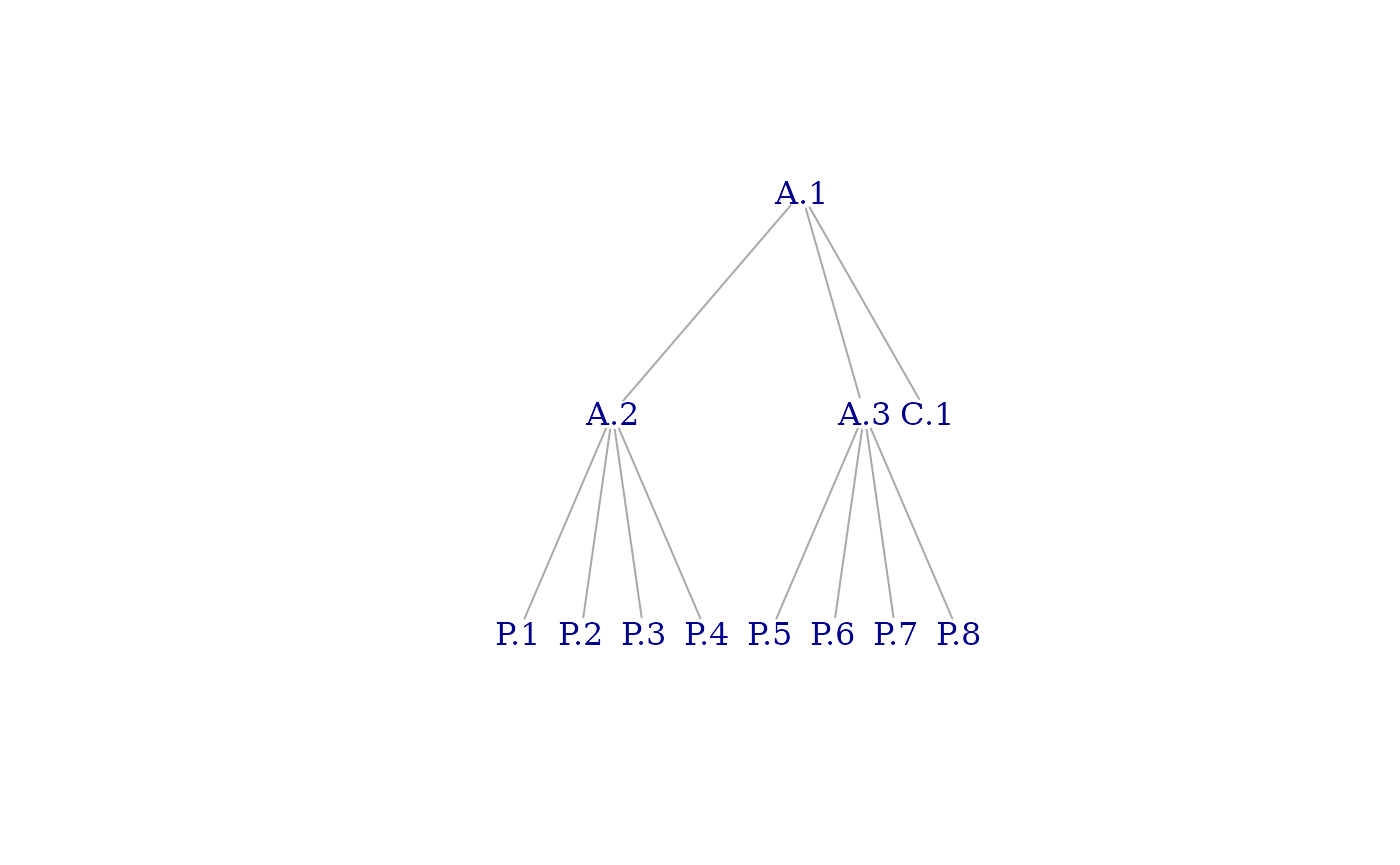
Then we can compute mass properties for non-leaf elements by calling rollup_mass_props():

rollup_mass_props(test_tree, test_table)
#>     id parent mass Cx Cy Cz Ixx  Ixy   Ixz Iyy   Iyz Izz POIconv Ipoint
#> 1  A.1          21  0  0  0 144 -4.8 -24.8 144 -23.2 139       -  FALSE
#> 2  A.2    A.1    8  1  0  0  32 -0.4  -0.4  24   0.4  24       -  FALSE
#> 3  A.3    A.1    8 -1  0  0  32 -0.4  -0.4  24   0.4  24       -  FALSE
#> 4  C.1    A.1    5  0  0  0  80 -4.0 -24.0  80 -24.0  75       -  FALSE
#> 5  P.1    A.2    2  1  1  1   4 -0.1  -0.1   4   0.1   4       -  FALSE
#> 6  P.2    A.2    2  1  1 -1   4 -0.1  -0.1   4   0.1   4       -  FALSE
#> 7  P.3    A.2    2  1 -1  1   4 -0.1  -0.1   4   0.1   4       -  FALSE
#> 8  P.4    A.2    2  1 -1 -1   4 -0.1  -0.1   4   0.1   4       -  FALSE
#> 9  P.5    A.3    2 -1  1  1   4 -0.1  -0.1   4   0.1   4       -  FALSE
#> 10 P.6    A.3    2 -1  1 -1   4 -0.1  -0.1   4   0.1   4       -  FALSE
#> 11 P.7    A.3    2 -1 -1  1   4 -0.1  -0.1   4   0.1   4       -  FALSE
#> 12 P.8    A.3    2 -1 -1 -1   4 -0.1  -0.1   4   0.1   4       -  FALSE

Note that, although the table shows the parent of each element for clarity of exposition, the child-parent relations are coneveyed only by the tree passed as the first argument.

The input may also contain uncertainties data. This example is from the Society of Allied Weight Engineers:

sawe_input
#>         id  mass    Cx    Cy    Cz     Ixx     Iyy      Izz    Ixy      Ixz
#> 1   Widget 57.83 121.2  0.04 -0.16 7258.90 8607.02 10453.40 834.44 -1198.38
#> 2 2nd Part 16.80  70.9 -0.95  0.46   65.07 1124.65  1078.82  76.01   202.83
#> 3 Combined    NA    NA    NA    NA      NA      NA       NA     NA       NA
#>        Iyz sigma_mass sigma_Cx sigma_Cy sigma_Cz sigma_Ixx sigma_Iyy sigma_Izz
#> 1 -1066.58     1.2416   0.2764   0.2085   0.0669  386.9233  171.4792  414.5547
#> 2    13.62     1.7308   0.6234   0.5173   0.1405   12.4687  109.1324  108.5481
#> 3       NA         NA       NA       NA       NA        NA        NA        NA
#>   sigma_Ixy sigma_Ixz sigma_Iyz Ipoint POIconv
#> 1 1440.5402  344.6237  124.6860  FALSE       +
#> 2   55.8879  212.1241   11.5408  FALSE       +
#> 3        NA        NA        NA  FALSE       +

rollup_mass_props_and_unc(sawe_tree, sawe_input)
#>         id  mass       Cx         Cy          Cz      Ixx      Iyy      Izz
#> 1   Widget 57.83 121.2000  0.0400000 -0.16000000 7258.900  8607.02 10453.40
#> 2 2nd Part 16.80  70.9000 -0.9500000  0.46000000   65.070  1124.65  1078.82
#> 3 Combined 74.63 109.8769 -0.1828594 -0.02043146 7341.733 42673.75 44482.05
#>        Ixy       Ixz       Iyz sigma_mass sigma_Cx  sigma_Cy   sigma_Cz
#> 1  834.440 -1198.380 -1066.580    1.24160  0.27640 0.2085000 0.06690000
#> 2   76.010   202.830    13.620    1.73080  0.62340 0.5173000 0.14050000
#> 3 1558.714 -1401.534 -1060.951    2.13008  0.95821 0.1999847 0.06178402
#>   sigma_Ixx sigma_Iyy sigma_Izz sigma_Ixy sigma_Ixz sigma_Iyz Ipoint POIconv
#> 1  386.9233  171.4792  414.5547 1440.5402  344.6237  124.6860  FALSE       +
#> 2   12.4687  109.1324  108.5481   55.8879  212.1241   11.5408  FALSE       +
#> 3  387.4017 2789.3133 2815.3260 1488.0948  418.6048  125.3175  FALSE       +

Objectives and Strategy

The objective of this package is to provide a trustworthy, well-documented, reference implementation for computation of mass properties (and their uncertainties) of aggregate objects from those of their parts. Aggregation can be recursive (e.g., indentured Bill of Materials), so it must accommodate trees of arbitrary depth and shape.

Strategies for achieving the objective include

• basing the calculations on published industry references,

• re-casting those lengthy reference equations into concise vector or matrix forms to reduce the error surface for source code and exploit the capabilities of R, which treats vectors and matrices as first-class objects,

• delegating orchestration to the rollupTree package, which, among other things, verifies that the input tree is well-formed and ensures proper ordering of computations,

• ensuring that all asserted leaf mass properties and uncertainties correspond to physically-realizable objects,

• coding in pure functional style, (i.e., avoiding mutable variables, implying iteration with Map() and Reduce()), and

• covering the entire code base with unit tests.

The author has intentionally made no effort to micro-optimize for performance. In particular, the author is aware that representing the inertia and its uncertainty as 3 ⨉ 3 matrices is “inefficient” to the degree that it independently calculates values that are redundant by symmetry. “Inefficient”, however, does not mean “slow”. See Performance Evaluation below.

Theory

In this section, we state the reference equations (Zimmerman and Nakai 2005) and show, where applicable, how those equations can be rewritten in more concise form. The form of the equations actually implemented is displayed within a box, e.g. $\boxed{F = ma}$.

The reference uses the word weight and the symbol $w$ in equations. We interpret weight as mass. The reference refers to center of mass by its $x$, $y$, and $z$ components. Symbols for moments ($I_{XX}$) and products ($I_{XY}$) of inertia are conventional. Variables with $i$ subscripts designate properties of parts; those without designate properties of aggregates. The letter $\sigma$ denotes uncertainty. $\sigma_w$, for example, is the mass uncertainty.

Mass Properties

Mass

The mass equation is suitable as is.

$$\boxed{ w = \sum_{i=1}^{n}w_i }$$

The corresponding R code is

  amp$mass <- Reduce(`+`, Map(f = function(mp) mp$mass, mpl))

In this and the following code snippets, the variable mpl is a list of input mass property sets for parts, the variable mp is a formal parameter of an anonymous function applied to each member of mpl, and amp is the resulting aggregate mass property set. The line above is an R functional programming idiom for “set the mass value of the aggregate to the sum of the mass values of the parts”.

Center of Mass

$$\begin{align} \bar{x} & = \sum_{i=1}^{n}{w_i}{{x}_i} \bigg/ \sum_{i=1}^{n}w_i\\ \bar{y} & = \sum_{i=1}^{n}{w_i}{{y}_i} \bigg/ \sum_{i=1}^{n}w_i\\ \bar{z} & = \sum_{i=1}^{n}{w_i}{{z}_i} \bigg/ \sum_{i=1}^{n}w_i\\ \end{align}$$

We can express center of mass as a 3-vector:

$$\boxed{ \begin{align} \boldsymbol{c}_i & = (x_i \quad y_i \quad z_i)^T \\ \boldsymbol{\bar{c}}& = (\bar{x} \quad \bar{y} \quad \bar{z})^T \end{align} }$$

Then

$$\boxed{ \boldsymbol{\bar{c}} = \frac{1}{w} \sum_{i=1}^{n}{w_i}{{\boldsymbol{c}}_i} }$$

The corresponding R code is

  amp$center_mass <- Reduce(`+`, Map(f = function(mp) mp$mass * mp$center_mass, mpl)) / amp$mass

Inertia Tensor

Moments of Inertia

$$\begin{align} I_{XX}& = \sum_{i=1}^{n} \left[ {I_{XX}}_i + w_i \left( {y}_i^2 + {z}_i^2 \right) - w_i \left( \bar{y}^2 + \bar{z}^2 \right) \right] & = \sum_{i=1}^{n} \left\{ {I_{XX}}_i + w_i \left[ \left( {y}_i - \bar{y} \right)^2 + \left( {z}_i - \bar{z} \right)^2 \right] \right\} \\ I_{YY}& = \sum_{i=1}^{n} \left[ {I_{YY}}_i + w_i \left( {x}_i^2 + {z}_i^2 \right) - w_i \left( \bar{x}^2 + \bar{z}^2 \right) \right] & = \sum_{i=1}^{n} \left\{ {I_{YY}}_i + w_i \left[ \left( {x}_i - \bar{x} \right)^2 + \left( {z}_i - \bar{z} \right)^2 \right] \right\} \\ I_{ZZ}& = \sum_{i=1}^{n} \left[ {I_{ZZ}}_i + w_i \left( {x}_i^2 + {y}_i^2 \right) - w_i \left( \bar{x}^2 + \bar{y}^2 \right) \right] & = \sum_{i=1}^{n} \left\{ {I_{ZZ}}_i + w_i \left[ \left( {x}_i - \bar{x} \right)^2 + \left( {y}_i - \bar{y} \right)^2 \right] \right\} \\ \end{align}$$

Products of Inertia

$$\begin{align} I_{XY}& = \sum_{i=1}^{n} \left[ {I_{XY}}_i + w_i {{x}_i}{{y}_i} -w_i (\bar{x}\bar{y})\right] & = \sum_{i=1}^{n} \left[ {I_{XY}}_i + w_i ({x}_i - \bar{x})({y}_i - \bar{y})\right] \\ I_{XZ}& = \sum_{i=1}^{n} \left[ {I_{XZ}}_i + w_i {{x}_i}{{z}_i} -w_i (\bar{x}\bar{z})\right] & = \sum_{i=1}^{n} \left[ {I_{XZ}}_i + w_i ({x}_i - \bar{x})({z}_i - \bar{z})\right] \\ I_{YZ}& = \sum_{i=1}^{n} \left[ {I_{YZ}}_i + w_i {{y}_i}{{z}_i} -w_i (\bar{y}\bar{z})\right] & = \sum_{i=1}^{n} \left[ {I_{YZ}}_i + w_i ({y}_i - \bar{y})({z}_i - \bar{z})\right] \\ \end{align}$$

Matrix Formulation

Let $\boldsymbol{I}$ be the inertia tensor of the aggregate and $\boldsymbol{I}_i$ be that of part $i$. The equations for products of inertia above clearly follow the positive integral convention, so

$$\boldsymbol{I} = \left[ \begin{array}{rrr} I_{XX}& -I_{XY}& -I_{XZ}\\ -I_{XY}& I_{YY}& -I_{YZ}\\ -I_{XZ}& -I_{YZ}& I_{ZZ}\\ \end{array} \right]$$

and similarly for $\boldsymbol{I}_i$.

Noting the repeated appearance of terms of the form $({x}_i - \bar{x})({y}_i - \bar{y})$, we form the outer product

$$\boxed{ \begin{align} \boldsymbol{d}_i & = (({x}_i - \bar{x}) \quad ({y}_i - \bar{y}) \quad ({z}_i - \bar{z}))^T \\ \boldsymbol{Q}_i & = \boldsymbol{d}_i {\boldsymbol{d}_i}^T \end{align} }$$ Then

$$\begin{align} \boldsymbol{Q}_i & = \begin{bmatrix} ({x}_i - \bar{x})^2 & ({x}_i - \bar{x})({y}_i - \bar{y}) & ({x}_i - \bar{x})({z}_i - \bar{z}) \\ ({y}_i - \bar{y})({x}_i - \bar{x}) & ({y}_i - \bar{y})^2 & ({y}_i - \bar{y})({z}_i - \bar{z}) \\ ({z}_i - \bar{z})({x}_i - \bar{x}) & ({z}_i - \bar{z})({y}_i - \bar{y}) & ({z}_i - \bar{z})^2 \\ \end{bmatrix} \end{align}$$

Let $\boldsymbol{s}_i$ be the matrix of inertia tensor summands from the reference equations. That is,

$$\boldsymbol{I} = \sum_{i=1}^{n} \boldsymbol{s}_i$$

where $$\begin{align} \boldsymbol{s}_i & = \boldsymbol{I}_i \\ & - w_i \begin{bmatrix} -({y}_i - \bar{y})^2 - ({z}_i - \bar{z})^2 & ({x}_i - \bar{x})({y}_i - \bar{y}) & ({x}_i - \bar{x})({z}_i - \bar{z}) \\ ({x}_i - \bar{x})({y}_i - \bar{y}) & -({x}_i - \bar{x})^2 - ({z}_i - \bar{z})^2 & ({y}_i - \bar{y})({z}_i - \bar{z}) \\ ({x}_i - \bar{x})({z}_i - \bar{z}) & ({y}_i - \bar{y})({z}_i - \bar{z}) & -({x}_i - \bar{x})^2 - ({y}_i - \bar{y})^2 \\ \end{bmatrix} \\ & = \boldsymbol{I}_i \\ & - w_i \begin{bmatrix} ({x}_i - \bar{x})^2 & ({x}_i - \bar{x})({y}_i - \bar{y}) & ({x}_i - \bar{x})({z}_i - \bar{z}) \\ ({x}_i - \bar{x})({y}_i - \bar{y}) & ({y}_i - \bar{y})^2 & ({y}_i - \bar{y})({z}_i - \bar{z}) \\ ({x}_i - \bar{x})({z}_i - \bar{z}) & ({y}_i - \bar{y})({z}_i - \bar{z}) & ({z}_i - \bar{z})^2 \\ \end{bmatrix} \\ & - w_i \begin{bmatrix} -({x}_i - \bar{x})^2 - ({y}_i - \bar{y})^2 - ({z}_i - \bar{z})^2 & 0 & 0 \\ 0 & -({x}_i - \bar{x})^2 - ({y}_i - \bar{y})^2 - ({z}_i - \bar{z})^2 & 0 \\ 0 & 0 &-({x}_i - \bar{x})^2 - ({y}_i - \bar{y})^2 - ({z}_i - \bar{z})^2 \\ \end{bmatrix} \\ & = \boldsymbol{I}_i - w_i \left( \boldsymbol{Q}_i - \mathrm{tr}(\boldsymbol{Q}_i) \boldsymbol{1}_3 \right) \end{align}$$

where $\mathrm{tr}(\boldsymbol{Q}_i)$ is the trace of $\boldsymbol{Q}_i$, i.e., the sum of its diagonal elements, and $\boldsymbol{1}_3$ is the 3⨉3 identity matrix. Therefore

$$\boxed{ \boldsymbol{I} = \sum_{i=1}^{n} \left( \boldsymbol{I}_i - w_i \boldsymbol{M}_i \right) }$$ where

$$\boxed{ \boldsymbol{M}_i = \boldsymbol{Q}_i - \mathrm{tr}(\boldsymbol{Q}_i) \boldsymbol{1}_3 }$$

The corresponding R code is

  amp$inertia <- Reduce(`+`, Map(
    f  = function(mp) {
      d <- amp$center_mass - mp$center_mass
      Q <- outer(d, d)
      M <- Q - sum(diag(Q)) * diag(3)
      if (mp$point) -mp$mass * M else mp$inertia - mp$mass * M
    },
    mpl
  ))

Mass Property Uncertainties

Mass Uncertainty

The mass uncertainty equation is suitable as is.

$$\boxed{ \sigma_w = \sqrt{ \sum_{i=1}^n {{\sigma_w}_i}^2 } }$$

The corresponding R code is

  amp$sigma_mass = sqrt(Reduce(`+`, Map(f = function(mp) mp$sigma_mass^2, mpl)))

Center of Mass Uncertainty

$$\begin{align} \sigma_\bar{x} & = \sqrt{ \sum_{i=1}^n \left\{ (w_i {{\sigma_\bar{x}}}_i)^2 + [{\sigma_w}_i ({x}_i - \bar{x})]^2 \right\} } \bigg/ \sum_{i=1}^{n}w_i \\ \\ \sigma_\bar{y} & = \sqrt{ \sum_{i=1}^n \left\{ (w_i {{\sigma_\bar{y}}}_i)^2 + [{\sigma_w}_i ({y}_i - \bar{y})]^2 \right\} } \bigg/ \sum_{i=1}^{n}w_i \\ \\ \sigma_\bar{z} & = \sqrt{ \sum_{i=1}^n \left\{ (w_i {{\sigma_\bar{z}}}_i)^2 + [{\sigma_w}_i ({z}_i - \bar{z})]^2 \right\} } \bigg/ \sum_{i=1}^{n}w_i \\ \\ \end{align}$$

As before, we create a 3-vector for center of mass uncertainties. Let

$$\boxed{ \begin{align} \boldsymbol{\sigma_c} & = (\sigma_\bar{x} \quad \sigma_\bar{y} \quad \sigma_\bar{z})^T \\ {\boldsymbol{\sigma_c}}_i & = ({\sigma_\bar{x}}_i \quad {\sigma_\bar{y}}_i \quad {\sigma_\bar{z}}_i)^T \end{align} }$$

If we construe (as R does) squaring and taking square roots of vectors element-wise, then

$$\boxed{ \boldsymbol{\sigma_c} = \frac{1}{w} \sqrt{ \sum_{i=1}^n \left\{ (w_i {{\boldsymbol{\sigma_c}}}_i)^2 + [{\sigma_w}_i ({\boldsymbol{c}}_i - \bar{\boldsymbol{c}})]^2 \right\}} }$$

The corresponding R code is

  amp$sigma_center_mass = sqrt(Reduce(`+`, Map(
    f = function(mp) {
      (mp$mass * mp$sigma_center_mass)^2 +
        (mp$sigma_mass * (mp$center_mass - amp$center_mass))^2
    },
    mpl
  ))) / amp$mass

Inertia Tensor Uncertainty

Moments of Inertia Uncertainties

$$\begin{align} \sigma_{I_{XX}} & = \sqrt{ \sum_{i=1}^n \left\{ \sigma_{{I_{XX}}_i}^2 + \left[ 2 w_i ({y}_i - \bar{y}) \sigma_{{y}_i} \right]^2 + \left[ 2 w_i ({z}_i - \bar{z}) \sigma_{{z}_i} \right]^2 + \left[ \left(({y}_i - \bar{y})^2 + ({z}_i - \bar{z})^2 \right)\sigma_{w_i}\right]^2 \right\} } \\ \sigma_{I_{YY}} & = \sqrt{ \sum_{i=1}^n \left\{ \sigma_{{I_{YY}}_i}^2 + \left[ 2 w_i ({x}_i - \bar{x}) \sigma_{{x}_i} \right]^2 + \left[ 2 w_i ({z}_i - \bar{z}) \sigma_{{z}_i} \right]^2 + \left[ \left(({x}_i - \bar{x})^2 + ({z}_i - \bar{z})^2 \right)\sigma_{w_i}\right]^2 \right\} } \\ \sigma_{I_{ZZ}} & = \sqrt{ \sum_{i=1}^n \left\{ \sigma_{{I_{ZZ}}_i}^2 + \left[ 2 w_i ({x}_i - \bar{x}) \sigma_{{x}_i} \right]^2 + \left[ 2 w_i ({y}_i - \bar{y}) \sigma_{{y}_i} \right]^2 + \left[ \left(({x}_i - \bar{x})^2 + ({y}_i - \bar{y})^2 \right)\sigma_{w_i}\right]^2 \right\} } \\ \end{align}$$

Products of Inertia Uncertainties

$$\begin{align} \sigma_{I_{XY}} & = \sqrt{ \sum_{i=1}^n \left\{ \sigma_{{I_{XY}}_i}^2 + \left[ ({x}_i - \bar{x}) w_i \sigma_{{y}_i}\right]^2 + \left[ ({x}_i - \bar{x})({y}_i - \bar{y})\sigma_{w_i} \right]^2 + \left[ ({y}_i - \bar{y}) w_i \sigma_{{x}_i} \right]^2 \right\} } \\ \sigma_{I_{XZ}} & = \sqrt{ \sum_{i=1}^n \left\{ \sigma_{{I_{XZ}}_i}^2 + \left[ ({x}_i - \bar{x}) w_i \sigma_{{z}_i}\right]^2 + \left[ ({x}_i - \bar{x})({z}_i - \bar{z})\sigma_{w_i} \right]^2 + \left[ ({z}_i - \bar{z}) w_i \sigma_{{x}_i} \right]^2 \right\} } \\ \sigma_{I_{YZ}} & = \sqrt{ \sum_{i=1}^n \left\{ \sigma_{{I_{YZ}}_i}^2 + \left[ ({y}_i - \bar{y}) w_i \sigma_{{z}_i}\right]^2 + \left[ ({y}_i - \bar{y})({z}_i - \bar{z})\sigma_{w_i} \right]^2 + \left[ ({z}_i - \bar{z}) w_i \sigma_{{y}_i} \right]^2 \right\} } \\ \end{align}$$

Matrix Formulation

Let

$$\boxed{ \begin{align} \boldsymbol{d}_i & = (({x}_i - \bar{x}) \quad ({y}_i - \bar{y}) \quad ({z}_i - \bar{z}))^T \\ {\boldsymbol{\sigma_c}}_i & = ({\sigma_\bar{x}}_i \quad {\sigma_\bar{y}}_i \quad {\sigma_\bar{z}}_i)^T \\ \boldsymbol{P}_i & = \boldsymbol{d}_i {\boldsymbol{\sigma_c}}_i^T \\ \boldsymbol{Q}_i & = \boldsymbol{d}_i {\boldsymbol{d}_i}^T \end{align} }$$

Then

$$\begin{align} \boldsymbol{P}_i & = \begin{bmatrix} ({x}_i - \bar{x})\sigma_{x_i} &({x}_i - \bar{x})\sigma_{y_i} &({x}_i - \bar{x})\sigma_{z_i} \\ ({y}_i - \bar{y})\sigma_{x_i} & ({y}_i - \bar{y})\sigma_{y_i} & ({y}_i - \bar{y})\sigma_{z_i} \\ ({z}_i - \bar{z})\sigma_{x_i} & ({z}_i - \bar{z})\sigma_{y_i} & ({z}_i - \bar{z})\sigma_{z_i} \\ \end{bmatrix} \\ \\ \boldsymbol{Q}_i & = \begin{bmatrix} ({x}_i - \bar{x})^2 &({x}_i - \bar{x})({y}_i - \bar{y}) &({x}_i - \bar{x})({z}_i - \bar{z}) \\ ({y}_i - \bar{y})({x}_i - \bar{x}) & ({y}_i - \bar{y})^2 & ({y}_i - \bar{y})({z}_i - \bar{z}) \\ ({z}_i - \bar{z})({x}_i - \bar{x}) & ({z}_i - \bar{z})({y}_i - \bar{y}) & ({z}_i - \bar{z})^2 \\ \end{bmatrix} \end{align}$$

Let $\boldsymbol{s}_i^2$ be the matrix of inertia tensor uncertainty summands in the standard formulas for a given subcomponent $i$ above. That is,

$$\boldsymbol{\sigma_I}^2 = \sum_{i=1}^{n} \boldsymbol{s}_i^2$$

Let ${p_X}_i$, ${p_Y}_i$, and ${p_Z}_i$ be the respective diagonal elements of $P_i$. Let $\boldsymbol{1}_3$ be the 3 ⨉ 3 identity matrix. If we interpret squaring a matrix as the Hadamard (element-wise) product with itself, then $$\begin{align} \boldsymbol{s}_i^2 & = {\boldsymbol{\sigma_I}}_i^2 \\ & + \begin{bmatrix} 2 w_i ({y}_i - \bar{y}) \sigma_{y_i} & w_i({x}_i - \bar{x}) \sigma_{y_i} & w_i({x}_i - \bar{x}) \sigma_{z_i} \\ w_i({x}_i - \bar{x}) \sigma_{y_i} & 2 w_i({x}_i - \bar{x}) \sigma_{x_i} & w_i ({y}_i - \bar{y}) \sigma_{z_i} \\ w_i({x}_i - \bar{x}) \sigma_{z_i} & w_i ({y}_i - \bar{y}) \sigma_{z_i} & 2 w_i({x}_i - \bar{x}) \sigma_{x_i} \end{bmatrix}^2 \\ & + \begin{bmatrix} 2 w_i ({z}_i - \bar{z}) \sigma_{z_i} & w_i ({y}_i - \bar{y}) \sigma_{x_i} & w_i ({z}_i - \bar{z}) \sigma_{x_i} \\ w_i ({y}_i - \bar{y}) \sigma_{x_i} & 2 w_i ({z}_i - \bar{z}) \sigma_{z_i} & w_i ({z}_i - \bar{z}) \sigma_{y_i} \\ w_i ({z}_i - \bar{z}) \sigma_{x_i} & w_i ({z}_i - \bar{z}) \sigma_{y_i} & 2 w_i ({y}_i - \bar{y}) \sigma_{y_i} \end{bmatrix}^2 \\ & + \begin{bmatrix} (({y}_i - \bar{y})^2 + ({z}_i - \bar{z})^2)\sigma_{w_i} &({x}_i - \bar{x})({y}_i - \bar{y})\sigma_{w_i} &({x}_i - \bar{x})({z}_i - \bar{z})\sigma_{w_i} \\ ({y}_i - \bar{y})({x}_i - \bar{x})\sigma_{w_i} & (({x}_i - \bar{x})^2 + ({z}_i - \bar{z})^2)\sigma_{w_i} & ({y}_i - \bar{y})({z}_i - \bar{z})\sigma_{w_i} \\ ({z}_i - \bar{z})({x}_i - \bar{x})\sigma_{w_i} & ({z}_i - \bar{z})({y}_i - \bar{y})\sigma_{w_i} & (({x}_i - \bar{x})^2 + ({y}_i - \bar{y})^2)\sigma_{w_i} \\ \end{bmatrix}^2 \\ \\ & = {\boldsymbol{\sigma_I}}_i^2 \\ & + w_i^2 \left( \boldsymbol{P}_i - \begin{bmatrix} ({x}_i - \bar{x})\sigma_{x_i} - 2 ({y}_i - \bar{y})\sigma_{y_i} & 0 & 0 \\ 0 & ({y}_i - \bar{y})\sigma_{y_i} - 2({x}_i - \bar{x})\sigma_{x_i} & 0 \\ 0 & 0 & ({z}_i - \bar{z})\sigma_{y_i} - 2({x}_i - \bar{x})\sigma_{x_i} \\ \end{bmatrix} \right) ^2 \\ & + w_i^2 \left( \boldsymbol{P}_i^T - \begin{bmatrix} ({x}_i - \bar{x})\sigma_{x_i} - 2 ({z}_i - \bar{z})\sigma_{y_i} & 0 & 0 \\ 0 & ({y}_i - \bar{y})\sigma_{y_i} - 2 ({z}_i - \bar{z})\sigma_{z_i} & 0 \\ 0 & 0 & ({z}_i - \bar{z})\sigma_{y_i} - 2 ({y}_i - \bar{y})\sigma_{y_i} \\ \end{bmatrix} \right) ^2 \\ & + \sigma_{w_i}^2 \left( \boldsymbol{Q}_i - \mathrm{tr}(\boldsymbol{Q}_i)\boldsymbol{1}_3 \right)^2 \\ \\ & = {\boldsymbol{\sigma_I}}_i^2 \\ & + w_i^2 \left( \boldsymbol{P}_i - \begin{bmatrix} {p_X}_i - 2 {p_Y}_i & 0 & 0 \\ 0 & {p_Y}_i - 2 {p_X}_i & 0 \\ 0 & 0 & {p_Z}_i - 2 {p_X}_i \\ \end{bmatrix} \right) ^2 \\ & + w_i^2 \left( \boldsymbol{P}_i^T - \begin{bmatrix} {p_X}_i - 2{p_Z}_i & 0 & 0 \\ 0 & {p_Y}_i - 2 {p_Z}_i & 0 \\ 0 & 0 & {p_Z}_i - 2 {p_Y}_i \\ \end{bmatrix} \right) ^2 \\ & + \sigma_{w_i}^2 \left( \boldsymbol{Q}_i - \mathrm{tr}(\boldsymbol{Q}_i)\boldsymbol{1}_3 \right)^2 \end{align}$$

Finally,

$$\boxed{ \boldsymbol{\sigma_I} = \sqrt{ \sum_{i=1}^{n} {\left\{ {\boldsymbol{\sigma_I}}_i^2 +{\boldsymbol{M}_4}_i \right\}} } }$$

where

$$\boxed{ \begin{align} {\boldsymbol{M}_1}_i & = \boldsymbol{P}_i - \begin{bmatrix} {p_X}_i - 2{p_Y}_i & 0 & 0 \\ 0 & {p_Y}_i - 2{p_X}_i & 0 \\ 0 & 0 & 2{p_Z}_i - 2{p_X}_i \\ \end{bmatrix} \\ {\boldsymbol{M}_2}_i & = \boldsymbol{P}_i^T - \begin{bmatrix} {p_X}_i - 2{p_Z}_i & 0 & 0 \\ 0 & {p_Y}_i - 2{p_Z}_i & 0 \\ 0 & 0 & 2{p_Z}_i - 2{p_Y}_i \\ \end{bmatrix} \\ {\boldsymbol{M}_3}_i & = \boldsymbol{Q}_i - \mathrm{tr}(\boldsymbol{Q}_i)\boldsymbol{1}_3 \\ {\boldsymbol{M}_4}_i & = w_i^2 \left( {{\boldsymbol{M}_1}_i}^2 + {{\boldsymbol{M}_2}_i}^2 \right) + \left( \sigma_{w_i} {\boldsymbol{M}_3}_i \right)^2 \end{align} }$$

The corresponding R code is

  amp$sigma_inertia = sqrt(Reduce(`+`, Map(
    f = function(mp) {

      d <- mp$center_mass - amp$center_mass

      P <- outer(d, mp$sigma_center_mass)
      p <- diag(P)

      Q <- outer(d, d)

      M1 <-   P  - diag(p - 2 * p[c("y", "x", "x")])
      M2 <- t(P) - diag(p - 2 * p[c("z", "z", "y")])
      M3 <-   Q  - sum(diag(Q)) * diag(3)
      M4 <- mp$mass^2 * (M1^2 + M2^2) + (mp$sigma_mass * M3)^2

      if (mp$point) M4 else mp$sigma_inertia^2 + M4
    },
    mpl
  )))

Radii of Gyration and Their Uncertainties

By definition:

$$\begin{align} k_X& = \sqrt{I_{XX}/ w} \\ k_Y& = \sqrt{I_{YY}/ w} \\ k_Z& = \sqrt{I_{ZZ}/ w} \\ \end{align}$$ Let

$$\boxed{ \begin{align} \boldsymbol{k} & = (k_X\quad k_Y\quad k_Z)^T \\ \boldsymbol{I} & = (I_{XX}\quad I_{YY}\quad I_{ZZ})^T \end{align} }$$ Then

$$\boxed{ \boldsymbol{k} = \sqrt{ \boldsymbol{I} / w } }$$

The corresponding R code is

      rg <- get_mass_props(d, i)
      rg$radii_gyration <- sqrt(diag(rg$inertia) / rg$mass)

The SAWE reference gives equations for uncertainties of radii of gyration in recursive form, but as these radii are simply functions of moments of inertia and mass, we should be able to express their uncertainties in terms of uncertainties of moments of inertia and mass by applying standard uncertainty propagation theory (Wikipedia contributors 2024).

Let

$$\boxed{ \begin{align} \sigma_\boldsymbol{k} & = (\sigma_{k_X} \quad \sigma_{k_Y} \quad \sigma_{k_Z})^T \\ \sigma_\boldsymbol{I} & = (\sigma_{I_{XX}} \quad \sigma_{I_{YY}} \quad \sigma_{I_{ZZ}})^T \end{align} }$$ Then

$$\begin{align} {\sigma_\boldsymbol{k}}^2 & \approx \left( \frac{\partial \boldsymbol{k}}{\partial \boldsymbol{I}} \right)^2 {\sigma_\boldsymbol{I}}^2 + \left( \frac{\partial \boldsymbol{k}}{\partial w} \right)^2 {\sigma_w}^2 + 2 \frac{\partial \boldsymbol{k}}{\partial \boldsymbol{I}} \frac{\partial \boldsymbol{k}}{\partial w} \sigma_{\boldsymbol{I}w} \\ & \approx \left( \frac{1}{2 \sqrt{w \boldsymbol{I}}} \right)^2 {\sigma_\boldsymbol{I}}^2 + \left(\frac{- \sqrt{\boldsymbol{I}}}{2 w^{3/2}}\right)^2 {\sigma_w}^2 + 2 \left( \frac{1}{2 \sqrt{w \boldsymbol{I}}} \right) \left(\frac{- \sqrt{\boldsymbol{I}}}{2 w^{3/2}}\right) \sigma_{\boldsymbol{I}w} \\ & \approx \frac{1}{4 w \boldsymbol{I}} {\sigma_\boldsymbol{I}}^2 + \frac{\boldsymbol{I}}{4 w^3} {\sigma_w}^2 - \frac{1}{2 w^2} \sigma_{\boldsymbol{I}w} \\ \end{align}$$ where $\sigma_{\boldsymbol{I}w}$ is the covariance between $\boldsymbol{I}$ and $w$.

Let $W$ and $X$ be random variables such that

$$\begin{align} W & = \sum_{i=1}^{n} (w_i + {\epsilon_w}_i) \\ X & = \sum_{i=1}^{n} \left\{ {I_{XX}}_i + {\epsilon_I_{XX}}_i + (w_i + {\epsilon_w}_i) \left[ \left( {y}_i - \bar{y} \right)^2 + \left( {z}_i - \bar{z} \right)^2 \right] \right\} \\ \end{align}$$ where $E[{\epsilon_w}_i] = 0$ and $E[{\epsilon_I_{XX}}_i] = 0$ for all $i$, $E[{\epsilon_w}_i {\epsilon_w}_j] = 0$ and $E[{\epsilon_I_{XX}}_i {\epsilon_I_{XX}}_j] = 0$ for all $i \neq j$, and $E[{\epsilon_w}_i {\epsilon_I_{XX}}_j] = 0$ for all $i$ and $j$. It is clear from the linearity of $W$ and $X$ in $w_i$ and $I_{XX}_i$ that

$$E[W] = E \left[\sum_{i=1}^{n} (w_i + {\epsilon_w}_i) \right] = w + \sum_{i=1}^{n} {\epsilon_w}_i = w$$ and $$\begin{align} E[X] & = E \left[ \sum_{i=1}^{n} \left\{ {I_{XX}}_i + {\epsilon_{I_{XX}}}_i + (w_i + {\epsilon_w}_i) \left[ \left( {y}_i - \bar{y} \right)^2 + \left( {z}_i - \bar{z} \right)^2 \right] \right\} \right] \\ & = I_{XX}+ E \left[ \sum_{i=1}^{n} \left\{ {\epsilon_{I_{XX}}}_i + {\epsilon_w}_i \left[ \left( {y}_i - \bar{y} \right)^2 + \left( {z}_i - \bar{z} \right)^2 \right] \right\} \right] \\ & = I_{XX} \end{align}$$ Therefore,

$$\begin{align} \sigma_{I_{XX}w} & = E \left[ \left( W - E[W] \right) \left( X - E[X] \right)\right] \\ & = E \left[ \sum_{i=1}^{n} {\epsilon_w}_i \sum_{j=1}^{n} \left\{ {\epsilon_{I_{XX}}}_j + {\epsilon_w}_j \left[ \left( {y}_j - \bar{y} \right)^2 + \left( {z}_j - \bar{z} \right)^2 \right] \right\} \right] \\ & = \sum_{i=1}^{n} \sum_{j=1}^{n} E \left[ {\epsilon_w}_i \left\{ {\epsilon_{I_{XX}}}_j + {\epsilon_w}_j \left[ \left( {y}_j - \bar{y} \right)^2 + \left( {z}_j - \bar{z} \right)^2 \right] \right\} \right] \\ & = \sum_{i=1}^{n} E \left[ {\epsilon_w}^2_i \right] \left[ \left( {y}_i - \bar{y} \right)^2 + \left( {z}_i - \bar{z} \right)^2 \right] \\ & = \sum_{i=1}^{n} {\sigma_w}^2_i \left[ \left( {y}_i - \bar{y} \right)^2 + \left( {z}_i - \bar{z} \right)^2 \right] \\ \end{align}$$

Exploiting symmetry, let

$$\boxed{ \begin{align} \boldsymbol{d}_i & = (({x}_i - \bar{x}) \quad ({y}_i - \bar{y}) \quad ({z}_i - \bar{z}))^T \\ \boldsymbol{s}_i & = (\boldsymbol{d}_i^T\boldsymbol{d}_i \quad \boldsymbol{d}_i^T\boldsymbol{d}_i \quad \boldsymbol{d}_i^T\boldsymbol{d}_i)^T \\ \end{align} }$$

$$\begin{align} {\sigma_\boldsymbol{k}}^2 & \approx \frac{1}{4 w \boldsymbol{I}} {\sigma_\boldsymbol{I}}^2 + \frac{\boldsymbol{I}}{4 w^3} {\sigma_w}^2 - \frac{1}{2 w^2} \sum_{i=1}^{n} {\sigma_w}^2_i (\boldsymbol{s}_i - \boldsymbol{d}_i^2 ) \\ \end{align}$$ Therefore, we define

$$\boxed{ \begin{align} {\sigma_\boldsymbol{k}} & = \frac{1}{2} \sqrt{ \frac{1}{w \boldsymbol{I}} {\sigma_\boldsymbol{I}}^2 + \frac{\boldsymbol{I}}{w^3} {\sigma_w}^2 - \frac{2}{w^2} \sum_{i=1}^{n} {\sigma_w}^2_i (\boldsymbol{s}_i - \boldsymbol{d}_i^2 ) } \end{align} }$$

The corresponding R code is

      amp <- get_mass_props_and_unc(ds, target)
      I <- diag(amp$inertia)
      sigma_I <- diag(amp$sigma_inertia)
      amp$sigma_radii_gyration <- sqrt(
        sigma_I^2 / (amp$mass * I) + (I * amp$sigma_mass^2) / amp$mass^3 -
          2 / amp$mass^2 * Reduce(
            `+`,
            Map(
              f = function(s) {
                mp <- get_mass_props_and_unc(ds, s)
                d2 <- (mp$center_mass - amp$center_mass)^2
                mp$sigma_mass^2 * (sum(d2) - d2)
              },
              sources
            ),
            init = c(0, 0, 0)
          )
      ) / 2

Testing and Validation

Comparison With Independently-Calculated Results

In this section we will calculate the results for the SAWE example step by step and compare them with the package results. The inputs are:

#>         id  mass    Cx    Cy    Cz     Ixx     Iyy      Izz    Ixy      Ixz
#> 1   Widget 57.83 121.2  0.04 -0.16 7258.90 8607.02 10453.40 834.44 -1198.38
#> 2 2nd Part 16.80  70.9 -0.95  0.46   65.07 1124.65  1078.82  76.01   202.83
#>        Iyz sigma_mass sigma_Cx sigma_Cy sigma_Cz sigma_Ixx sigma_Iyy sigma_Izz
#> 1 -1066.58     1.2416   0.2764   0.2085   0.0669  386.9233  171.4792  414.5547
#> 2    13.62     1.7308   0.6234   0.5173   0.1405   12.4687  109.1324  108.5481
#>   sigma_Ixy sigma_Ixz sigma_Iyz Ipoint POIconv
#> 1 1440.5402  344.6237  124.6860  FALSE       +
#> 2   55.8879  212.1241   11.5408  FALSE       +

Our computed result is

t <- rollup_radii_of_gyration_unc(sawe_tree,
  add_radii_of_gyration(
    rollup_mass_props_and_unc(sawe_tree, sawe_table)
  )
)
sawe_result <- t[t$id == "Combined", ]
sawe_result
#>         id  mass       Cx         Cy          Cz      Ixx      Iyy      Izz
#> 3 Combined 74.63 109.8769 -0.1828594 -0.02043146 7341.733 42673.75 44482.05
#>        Ixy       Ixz       Iyz sigma_mass sigma_Cx  sigma_Cy   sigma_Cz
#> 3 1558.714 -1401.534 -1060.951    2.13008  0.95821 0.1999847 0.06178402
#>   sigma_Ixx sigma_Iyy sigma_Izz sigma_Ixy sigma_Ixz sigma_Iyz Ipoint POIconv
#> 3  387.4017  2789.313  2815.326  1488.095  418.6048  125.3175  FALSE       +
#>         kx       ky       kz  sigma_kx  sigma_ky  sigma_kz
#> 3 9.918422 23.91243 24.41382 0.2971248 0.5484836 0.5402033

Mass

mass <- sum(sawe_input$mass)

The independently-calculated mass is

#> [1] 74.63

This agrees with the computed result.

Center of Mass

C <- apply(sawe_input$mass / mass * sawe_input[, c("Cx", "Cy", "Cz")], 2, sum)

The independently-calculated center of mass is

#>           Cx           Cy           Cz 
#> 109.87693957  -0.18285944  -0.02043146

This agrees with the computed result.

Moments of Inertia

moi <- function(I, v1, v2, m, c1, c2) {
  sum(I + m * ((v1^2 + v2^2) - (c1^2 + c2^2)))
}
MOI <- c(
  Ixx = moi(sawe_input$Ixx, sawe_input$Cy, sawe_input$Cz, sawe_input$mass, C["Cy"], C["Cz"]),
  Iyy = moi(sawe_input$Iyy, sawe_input$Cx, sawe_input$Cz, sawe_input$mass, C["Cx"], C["Cz"]),
  Izz = moi(sawe_input$Izz, sawe_input$Cx, sawe_input$Cy, sawe_input$mass, C["Cx"], C["Cy"])
)

The independently-calculated moments of inertia are

#>       Ixx       Iyy       Izz 
#>  7341.733 42673.747 44482.052

This agrees with the computed result.

Products of Inertia

poi <- function(I, v1, v2, m, c1, c2) {
  sum(I + m * (v1 * v2 - c1 * c2))
}
POI <- c(
  Ixy = poi(sawe_input$Ixy, sawe_input$Cx, sawe_input$Cy, sawe_input$mass, C["Cx"], C["Cy"]),
  Ixz = poi(sawe_input$Ixz, sawe_input$Cx, sawe_input$Cz, sawe_input$mass, C["Cx"], C["Cz"]),
  Iyz = poi(sawe_input$Iyz, sawe_input$Cy, sawe_input$Cz, sawe_input$mass, C["Cy"], C["Cz"])
)

The independently-calculated products of inertia are

#>       Ixy       Ixz       Iyz 
#>  1558.714 -1401.534 -1060.951

This agrees with the computed result.

Radii of Gyration

rog <- function(I, m) sqrt(I / m)
ROG <- c(
  kx = rog(sawe_result$Ixx, sawe_result$mass),
  ky = rog(sawe_result$Iyy, sawe_result$mass),
  kz = rog(sawe_result$Izz, sawe_result$mass)
)

The independently-calculated radii of gyration are

#>        kx        ky        kz 
#>  9.918422 23.912428 24.413817

This agrees with the computed result.

Mass Uncertainty

sigma_mass <- sqrt(sum(sawe_input$sigma_mass^2))

The independently-calculated mass uncertainty is

#> [1] 2.13008

This agrees with the computed result.

Center of Mass Uncertainty

sigma_cm <- function(m, sigma_v, sigma_m, v, c, mass) {
  sqrt(sum((m * sigma_v)^2 + (sigma_m * (v - c))^2)) / mass
}
sigma_C <- c(
  sigma_Cx = sigma_cm(sawe_input$mass, sawe_input$sigma_Cx, sawe_input$sigma_mass, sawe_input$Cx, C["Cx"], mass),
  sigma_Cy = sigma_cm(sawe_input$mass, sawe_input$sigma_Cy, sawe_input$sigma_mass, sawe_input$Cy, C["Cy"], mass),
  sigma_Cz = sigma_cm(sawe_input$mass, sawe_input$sigma_Cz, sawe_input$sigma_mass, sawe_input$Cz, C["Cz"], mass)
)

The independently-calculated center of mass uncertainties are

#>   sigma_Cx   sigma_Cy   sigma_Cz 
#> 0.95821004 0.19998470 0.06178402

This agrees with the computed result.

Moments of Inertia Uncertainties

sigma_moi <- function(sigma_I, mass, sigma_mass, v1, v2, c1, c2, sigma_v1, sigma_v2) {
  sqrt(sum(
    sigma_I^2 +
    (2 * mass * (v1 - c1) * sigma_v1)^2 +
    (2 * mass * (v2 - c2) * sigma_v2)^2 +
    (((v1 - c1)^2 + (v2 - c2)^2) * sigma_mass)^2
  ))
}
sigma_MOI <- c(
  sigma_Ixx = sigma_moi(sawe_input$sigma_Ixx, sawe_input$mass, sawe_input$sigma_mass, sawe_input$Cy,
                                  sawe_input$Cz, C["Cy"], C["Cz"], sawe_input$sigma_Cy, sawe_input$sigma_Cz),
  sigma_Iyy = sigma_moi(sawe_input$sigma_Iyy, sawe_input$mass, sawe_input$sigma_mass, sawe_input$Cx,
                                  sawe_input$Cz, C["Cx"], C["Cz"], sawe_input$sigma_Cx, sawe_input$sigma_Cz),
  sigma_Izz = sigma_moi(sawe_input$sigma_Izz, sawe_input$mass, sawe_input$sigma_mass, sawe_input$Cx,
                                  sawe_input$Cy, C["Cx"], C["Cy"], sawe_input$sigma_Cx, sawe_input$sigma_Cy)
)

The independently-calculated moments of inertia uncertainties are

#> sigma_Ixx sigma_Iyy sigma_Izz 
#>  387.4017 2789.3133 2815.3260

This agrees with the computed result.

Products of Inertia Uncertainties

sigma_poi <- function(sigma_I, mass, sigma_mass, v1, v2, c1, c2, sigma_v1, sigma_v2) {
  sqrt(sum(
    sigma_I^2 +
    ((v1 - c1) * mass * sigma_v2)^2 +
    ((v1 - c1) * (v2 - c2) * sigma_mass)^2 +
    ((v2 - c2) * mass * sigma_v1)^2
  ))
}
sigma_POI <- c(
  sigma_Ixy = sigma_poi(sawe_input$sigma_Ixy, sawe_input$mass, sawe_input$sigma_mass, sawe_input$Cx,
                                  sawe_input$Cy, C["Cx"], C["Cy"], sawe_input$sigma_Cx, sawe_input$sigma_Cy),
  sigma_Ixz = sigma_poi(sawe_input$sigma_Ixz, sawe_input$mass, sawe_input$sigma_mass, sawe_input$Cx,
                                  sawe_input$Cz, C["Cx"], C["Cz"], sawe_input$sigma_Cx, sawe_input$sigma_Cz),
  sigma_Iyz = sigma_poi(sawe_input$sigma_Iyz, sawe_input$mass, sawe_input$sigma_mass, sawe_input$Cy,
                                  sawe_input$Cz, C["Cy"], C["Cz"], sawe_input$sigma_Cy, sawe_input$sigma_Cz)
)

The independently-calculated products of inertia uncertainties are

#> sigma_Ixy sigma_Ixz sigma_Iyz 
#> 1488.0948  418.6048  125.3175

This agrees with the computed result.

Radii of Gyration Uncertainties

sigma_rog <- function(mt, It, sigma_mt, sigma_It, v1, c1, v2, c2, sigma_m) {
  sqrt(sigma_It^2 / (4 * mt * It) + (It * sigma_mt^2) / (4 * mt^3) - sum(sigma_m^2 * ((v1 - c1)^2 + (v2 - c2)^2)) / (2 * mt^2))
}
sigma_ROG <- c(
  sigma_kx = sigma_rog(sawe_result$mass, sawe_result$Ixx, sawe_result$sigma_mass, sawe_result$sigma_Ixx,
                       sawe_input$Cy, sawe_result$Cy, sawe_input$Cz, sawe_result$Cz, sawe_input$sigma_mass),
  sigma_ky = sigma_rog(sawe_result$mass, sawe_result$Iyy, sawe_result$sigma_mass, sawe_result$sigma_Iyy,
                       sawe_input$Cx, sawe_result$Cx, sawe_input$Cz, sawe_result$Cz, sawe_input$sigma_mass),
  sigma_kz = sigma_rog(sawe_result$mass, sawe_result$Izz, sawe_result$sigma_mass, sawe_result$sigma_Izz,
                       sawe_input$Cx, sawe_result$Cx, sawe_input$Cy, sawe_result$Cy, sawe_input$sigma_mass)
)

The independently-calculated radii of gyration uncertainties are

#>  sigma_kx  sigma_ky  sigma_kz 
#> 0.2971248 0.5484836 0.5402033

This agrees with the computed result.

Comparison With Published Results

The SAWE reference provides computed results for their example (excluding radii of gyration and their uncertainties). These results match those within a tolerance of 0.2%. The small differences are likely because their actual input values were not identical to the truncated values published in the article.

Performance Evaluation

mp_table and mp_tree are a synthesized data set representing a tree of depth 7 with 1765 vertices and 1764 edges. 1267 vertices are leaves, the remaining 498 are non-leaves. Rolling up mass properties and uncertainties for this data set combines 35280 input values to produce 9960 output values. Mass properties alone halves those values.

Benchmarks were taken on a platform with these CPU characteristics:

Python Version: 3.12.7.final.0 (64 bit)
Cpuinfo Version: 9.0.0
Vendor ID Raw:
Hardware Raw:
Brand Raw: Apple M3
Hz Advertised Friendly:
Hz Actual Friendly: 2.4000 GHz
Hz Advertised:
Hz Actual: (2400000000, 0)
Arch: ARM_8
Bits: 64
Count: 8
Arch String Raw: arm64
L1 Data Cache Size:
L1 Instruction Cache Size:
L2 Cache Size:
L2 Cache Line Size:
L2 Cache Associativity:
L3 Cache Size:
Stepping:
Model:
Family: 6
Processor Type:
Flags: acpi, aes, apic, clfsh, cmov, cx16, cx8, de, ds, dscpl, dtse64, est, fpu, fxsr, htt, mca, mce, mmx, mon, msr, mtrr, pae, pat, pbe, pclmulqdq, pdcm, pge, pse, pse36, seglim64, sep, ss, sse, sse2, sse3, sse4.1, sse4.2, ssse3, tm, tm2, tpr, tsc, vme, vmx

Benchmark results for rollup of mass properties and uncertainties were taken with and without input validation:

benchmark('mp + unc no validation' = rollup_mass_props_and_unc_fast(mp_tree, mp_table),
          'mp + unc    validation' = rollup_mass_props_and_unc(mp_tree, mp_table),
          'mp       no validation' = rollup_mass_props_fast(mp_tree, mp_table),
          'mp          validation' = rollup_mass_props(mp_tree, mp_table),
          replications = 10,
          columns = c("test", "replications", "elapsed", "user.self", "sys.self")
) |> mutate(elapsed = elapsed / 10, user.self = user.self / 10, sys.self = sys.self / 10)

Times reported are in seconds.

                    test replications elapsed user.self sys.self
4 mp          validation           10  1.0340    1.0182   0.0161
3 mp       no validation           10  0.6926    0.6821   0.0106
2 mp + unc    validation           10  1.6079    1.5814   0.0268
1 mp + unc no validation           10  1.0657    1.0465   0.0194

References

Wikipedia contributors. 2024. “Propagation of Uncertainty — Wikipedia, the Free Encyclopedia.” https://en.wikipedia.org/w/index.php?title=Propagation_of_uncertainty&oldid=1260292643.

Zimmerman, Robert L., and John H. Nakai. 2005. “Are You Sure? Uncertainty in Mass Properties Engineering.” In 64th Annual International Conference on Mass Properties Engineering, 123–60. Society of Allied Weight Engineers.